Transfer Learning with Keras

Transfer Learning is a very important concept in ML generally and DL specifically. It aims to reuse the knowledge gathered by an already trained model on a specific task and trasfer this knowledge to a new task. By doing this, the new model can be trained in less time and may also require less data compared to training a regular model from scratch.

The following article shows how easy it is to achieve “transfer learning” in the image classification task with Keras. Starting from a classifier trained on the ImageNet Dataset, we will re-adapt the classifier architecture to the problem of recognizing World Chess champions and traing the new model with few images. With such an approach we can train our model very fast (in a matter of seconds) with very few images (sometines a dozen can be enough) yet we will get a good accuracy. In fact, even if that there are no Chess champions images in ImageNet, it turns out that ImageNet is already good enough at recognizing things in the world.

Data

We will build a classifier that recognizes world Chess champions (or any other subject), so on google images, search for the names of champions. Then on the Developer Console, type the following javascript snipet to download urls of the displayed image in a CSV file:

urls = Array.from(document.querySelectorAll('.rg_di .rg_meta')).map(el=>JSON.parse(el.textContent).ou);
window.open('data:text/csv;charset=utf-8,' + escape(urls.join('\n')));

Download the pictures using the URLs you got from last step and store them in an imagenet compatible folder structure (with train, validation and test subsets), i.e.

root
|_ dataset
    |_ train
        |_ label1
        |_ label2
        |_ ...
    |_ test
        |_ label1
        |_ label2
        |_ ...

Model

We will take a ResNet-50 pre-trained model, and then we train it to predict our labels (i.e. World Chess champions). In keras, it’s simply:

from tensorflow.keras.applications.resnet50 import ResNet50

model1 = ResNet50(weights='imagenet')

For the moment we cannot use this model for our task, in fact if you look at the summary of this model with model1.summary(), it has a last layer with 1000 outputs. This is because the model was trained to recognize the categories available in ImageNet (i.e. 1000).

We need to readapt the model to our task by doing the following:

1. Remove the last layer of the original model.
2. Add a header on top of this base model with an output size same as the number of categories,
3. Freeze the layers in this base model, i.e. layer.trainable = False
4. Train only the head using the previous downloaded pictures of champions.

In Keras, the previous steps translates into:

x = model1.layers[-3].output                     # shape (bs, 7, 7, 2048)
x = Dropout(rate=0.3)(x)                         # shape (bs, 7, 7, 2048)
x = GlobalAveragePooling2D()(x)                  # shape (bs, 2048)
x = Dense(1024, activation='relu')(x)            # shape (bs, 1024)
x = BatchNormalization()(x)                      # shape (bs, 1024)
y = Dense(len(classes), activation='softmax')(x) # shape (bs, len(classes))

# create a new model with input similar to the base imagenet model and output as the predictions
model2 = Model(inputs=model1.input, outputs=y)

Then freezing the earlier layers from the original model, and training only the newly added layers as follows:

# freeze layers from base model
for layer in model1.layers:
    layer.trainable = False

# compile the new model
adam = Adam(lr=0.001, epsilon=0.01, decay=0.0001)
model2.compile(optimizer=adam, loss='categorical_crossentropy', metrics=['accuracy'])

# setup generators for train and validation set
train_dl = ImageGenerator(path, classes, batch_size=48)
valid_dl = ImageGenerator(path, classes, batch_size=48, validation=True)

# fit the model using the previous generators
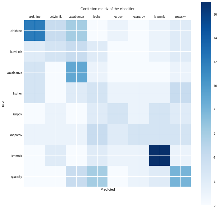
history = model2.fit_generator(generator=train_dl, validation_data=valid_dl, epochs=10, use_multiprocessing=True)

After traning the model, we can use Confusion matrix to analyze what classes where predicted well and which one where confusion for the trained model. E.g. in the following matrix Kramnik is well recognized by the model but it fails to properly distinguish fischer/karpov/kasparov. When looking at the dataset, many fischer images contain karpov as they played againts each other in the Match of the Century. Similarly for karpov and kasparov.

To visualy explain what the trained model look at in an input picture, we can use the Grad-CAM as follows:

# read an image from url
img = preprocessing.image.load_img(img_path, target_size=image_size)
img_data = preprocessing.image.img_to_array(img)
x = np.expand_dims(img_data, axis=0)
x = preprocess_input(x)

# get the activation of the last conv layer
target_layer_index = len(model2.layers) - 6 # activation_48
target_layer_output = K.function([model2.layers[0].input], [model2.layers[target_layer_index].output])
activations = target_layer_output([x])[0]   # shape (7, 7, 2048)
activations_avg = activations.mean(-1)[0]   # shape (7, 7)

# display the heatmap on top of the original image
_,ax = plt.subplots()
plt.xticks([], []); plt.yticks([], [])
ax.imshow(img)
ax.imshow(activations_avg, alpha=0.6, extent=(0,224,224,0), interpolation='bilinear', cmap='magma');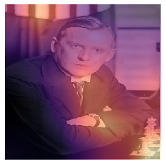

Further experiment

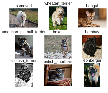
As a second experiment with Transfer Learning for image classification, applying the same approach on the Oxford-IIIT Pet Dataset which has 37 categories of dogs and cats, with 200 images for each class.

After only five epochs, we already get pretty good result with our classifier

Epoch 5/5
94/94 [==============================] - 64s 685ms/step - loss: 0.1128 - acc: 0.9835 - val_loss: 0.8669 - val_acc: 0.7520

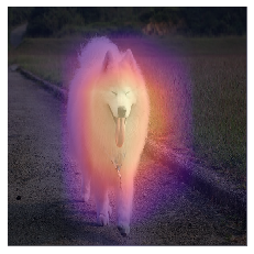
And looking at the heat map of the activation we can see that the classifier did a pretty good job at locating the important section in the image.

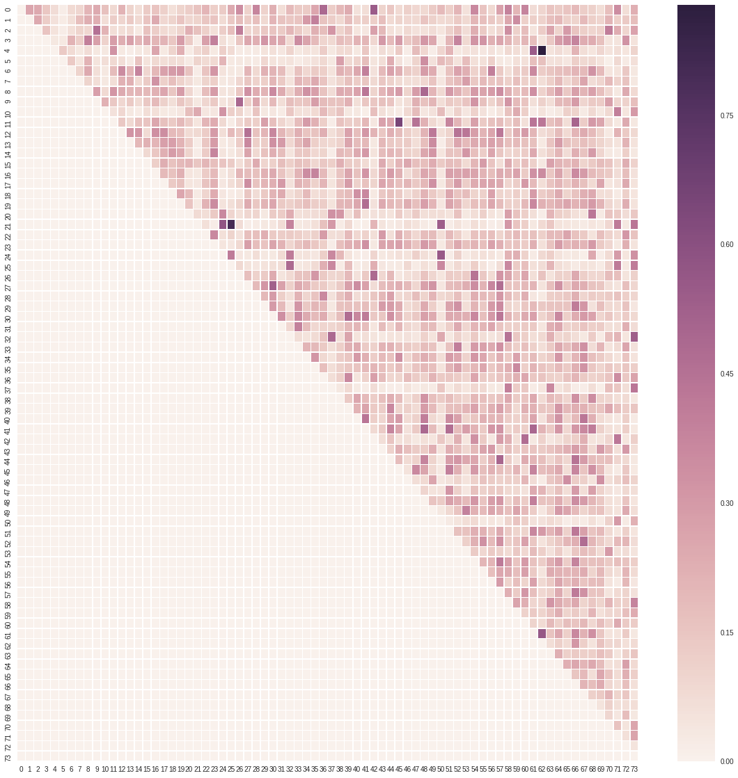
One we can also do to have better idea of the dataset is calculating the Cosine Similarity between few of the images. I took two images from each category and calculated the similarity in TensorFlow as follows:

a = tf.placeholder(tf.float32, shape=[None], name="input_placeholder_a")
b = tf.placeholder(tf.float32, shape=[None], name="input_placeholder_b")
normalize_a = tf.nn.l2_normalize(a,0)
normalize_b = tf.nn.l2_normalize(b,0)
cos_similarity=tf.reduce_sum(tf.multiply(normalize_a,normalize_b))
sess = tf.Session()
cos_sim = sess.run(cos_similarity,feed_dict={a:x1,b:x2})

Displaying the resulting matrix using Seaborn Heatmap gives the following picture:

What’s next

We can take this approach further by automating the process of re-adapting the NN architecture so that a user have to only pass the dataset and the system will infer the architecture.

Notebooks

World Chess Champions	Run notebook in Google Colab	view notebook on Github
Oxford-IIIT Pet Dataset	Run notebook in Google Colab	view notebook on Github