X Degrees of Separation with PyTorch

What is the connection between a 4000 year old clay figure and Van Gogh’s Starry Night? How do you get from Bruegel’s Tower of Babel to the street art of Rio de Janeiro? What links an African mask to a Japanese wood cut?

Google X Degrees of Separation (link) is an Artistic experiment made in collaboration by Google and artist Mario Klingemann. This online tool uses AI to build a path between two images so that the in between images constitue and natural jump from one image to the other until the final image.

The basic idea behind this tool, is to extract images features from the dataset and use these features to calculate the how close are each pair of images in the dataset (a.k.a Similarity). These distances are later used to build a graph with images as nodes connected with a weithed edge based on the distance between the two nodes. As a result, finding the shortest path between two images become a classic graph problem.

The following article describes a simple approach to implement X Degrees of Separation with PyTorch.

Data

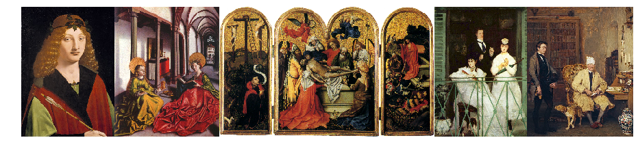
The data used is a subset from WikiArt Emotions dataset which is a subset of about 4000 visual arts from the WikiArt encyclopedia. The following is a sample from this dataset.

Strategy

The approach to the replicate the X Degrees of Separation tool is as follows:

1) Feature extraction:

Extract classification features from each image in the dataset by using an pre-trained model (on imagenet for instance) as follows:

# base model: imagenet classifier
model = models.resnet18(pretrained=True)
# feature extractor from the base model, up to the layer before average pooling
feature_modules = list(model.children())[:-2]
feature_extractor = nn.Sequential(*feature_modules)
# for every batch in the DataLoader
for batch in dataloader:
    # get the input (we don't need the labels)
    X, y = batch
    # run the model to get the image features
    preds = feature_extractor(X)
    # preds shape is: batch_size, 512, 4, 4 (i.e. output of the last BatchNorm layer)
    # avergare over the the last two dimensions
    features_batch = preds.mean(-1).mean(-1)

Then to speed up the calculation of distance between each image, apply a PCA to compress those features into orthogonal feautre vectors. So instead of a feature vector of 512 per image we end up with smaller vector (says dozen). Also PCA should be good at capturing most of the information in this new space.

The calculation of princial components is done simply as follows:

import fbpca
(U, s, Va) = fbpca.pca(features, k=10, raw=True, n_iter=10)
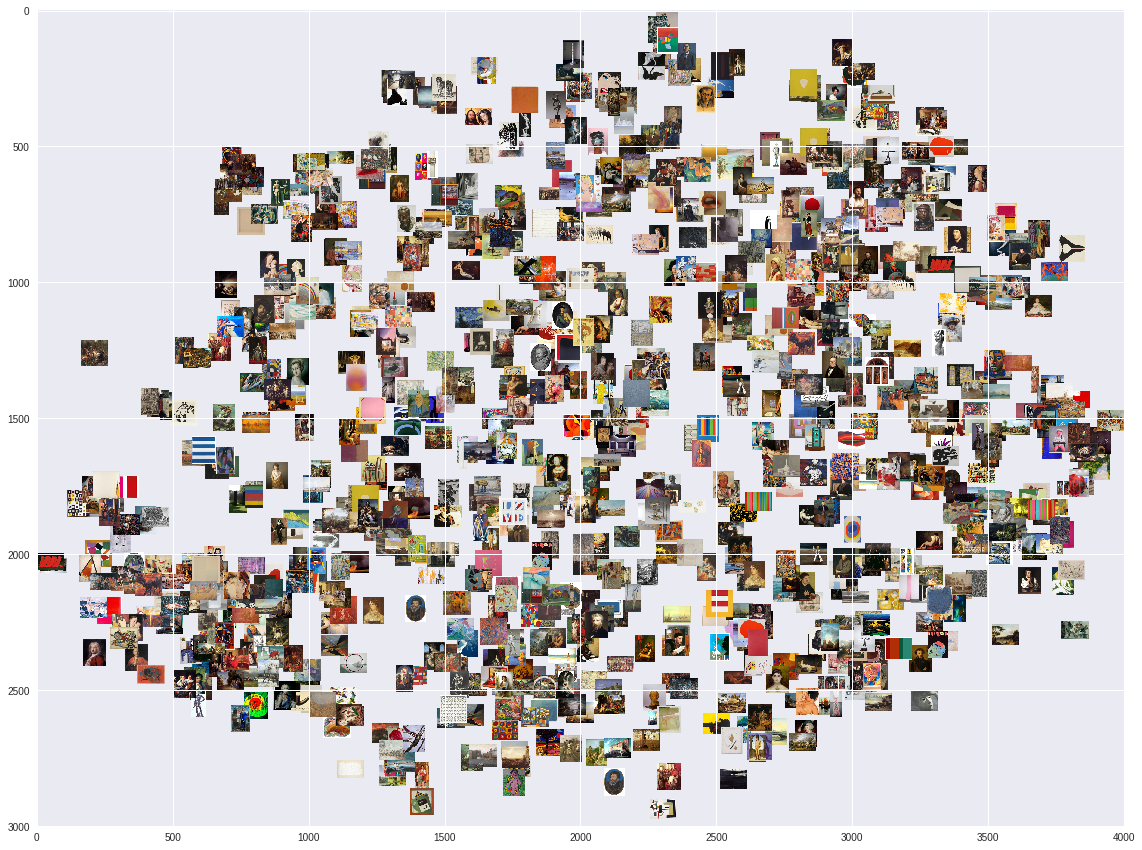
features_pca = U

Visualizing those images with t-SNE give somethning like the followings (it clearly shows that those images cannot be grouped into clusters using the given features):

2) Neighborhood Graph:

With the PCA features calculated for each image, we try to find the k neighboring images with the smallest cosine distance from it. Using the pretty fast NMSLIB, kNN are calculated as follows:

import nmslib
# Initializes a new index
index = nmslib.init(space='angulardist')
# Add the datapoints to the index
index.addDataPointBatch(features_pca)
# Create the index for querying
index.createIndex()
# nearest neighborhood on features array
nn_idxs, nn_dists = zip(*index.knnQueryBatch(features_pca, k=20, num_threads=4))

The calculated distances are used to build a graph with the images as nodes and nearest-neighbors as the edges connecting the nodes. Using the iGraph graph analysis library, this is achieved as follows:

from igraph import *
# create graph instance
g = Graph()
# create the vertices
g.add_vertices(dataset_size)
# create the edges for each element in the kNN distances array
for i in range(size):
    for j in range(1, k):
        g.add_edge(nn_idxs[i][0], nn_idxs[i][j], weight=nn_dists[i][j])

3) Runtime:

With the neighborhood graph at hand, we can for each pair of images (present in this graph), try to find a possible path between them. In this path, each consecutive pair of images are connected by a neighborhood connection. Using the iGraph API, finding shortest path is as simple as this:

g.get_shortest_paths(src, to=dst, mode=OUT, output='vpath', weights='weight')[0]

For instance applying this on two randomly selected images gives the following result (path is from left to right with the image to the left is source and the image to the right is the target)):

Conclusion

The advantage of such an approach is that it’s straightforward and pretty easy to implement. May be even fast then other approaches at run-time. This simplicity is also a disadvantage, using kNN with threshold doesn’t guarantee the existance of a path between every pair of two images. In fact this is why I grapped all neighboors wihtout applying a threshold durign the selection process. Also, in case of unevenly distributed image set, this approach may produce very densely connected clusters. Thus, some regions with high inner similarity can be isolated from the rest of the image space.

I guess more sophisticated approaches (will try to find some) could be used to ensure that edges do not become too long or too short and gurantee a uniform degree of separation between nodes.

Full notebook can be found here - link