
DeepLearning on Spark with Analytics Zoo and BigDL
22 Dec 2021 by dzlabAnalytics Zoo is an open source Deep Learning library. Along with BigDL, it allows to train and run Deep Learning workloads on Spark and Ray. Furthermore, this library has a Keras API which make using it very similar to using plain Keras API.
This articles shows how to use the Keras API to train and evaluate a classification model on the iris dataset. Furthermore, we will use TensorBoard to analyze training logs.
1. Add a dependency to Intel’s Analytics Zoo library which will bring in the jvm deep learning library BigDL.
libraryDependencies += "com.intel.analytics.zoo" % "analytics-zoo-bigdl_0.12.1-spark_3.0.0" % "0.9.0",
2. create a SparkSession and initialize Analytics Zoo context
val spark = SparkSession.builder().appName("analytics-zoo-demo").master("local[*]").getOrCreate()
val sc = NNContext.initNNContext(spark.sparkContext.getConf)
3. Read the raw data (in this case a CSV file containing the Iris dataset) into a Spark DataFrame
val path = getClass.getClassLoader.getResource("iris.csv").toString

val df = spark.read.option("header", true).option("inferSchema", true).csv(path)
4. Create a training dataset from the raw DataFrame
4.1. Define a helper function to transform each row into a Sample instance with:
- a tensor for the raining features
"sepal_len", "sepal_wid", "petal_len", "petal_wid"and - another tensor for the label
class.
def prepareDataset(df: DataFrame, labelColumn: String, featureColumns: Array[String]): RDD[Sample[Float]] = {
    val columns = trainDF.columns
    val labelIndex = columns.indexOf(labelColumn)
    val featureIndices = featureColumns.map(fc => df.columns.indexOf(fc))
    val dimInput = featureColumns.length
    df.rdd.map{row =>
      val features = featureIndices.map(row.getDouble(_).toFloat)
      val featureTensor = Tensor[Float](features, Array(dimInput))
      val labelTensor = Tensor[Float](1)
      labelTensor(Array(1)) = labels.indexOf(row.getString(labelIndex)) + 1
      Sample[Float](featureTensor, labelTensor)
    }
}
4.2. Apply the helper function on the training and validation datasets
val labels = Array("Iris-setosa", "Iris-versicolor", "Iris-virginica")
val labelCol = "class"
val featureCols = Array("sepal_len", "sepal_wid", "petal_len", "petal_wid")
val (trainDF, validDF, evalDF) = dataset.randomSplit(Array(0.8, 0.1, 0.1), 31)
val trainRDD = prepareDatasetForFitting(trainDF, labelCol, featureCols)
val validRDD = prepareDatasetForFitting(validDF, labelCol, featureCols)
val evalRDD = prepareDatasetForFitting(evalDF, labelCol, featureCols)
5. Create the model architecture by definining the list of layers and their respective activation functions.
val dimInput = 4
val dimOutput = 3
val nHidden = 100
val model = Sequential[Float]()
model.add(Dense[Float](nHidden, activation = "relu", inputShape = Shape(dimInput)).setName("fc_1"))
model.add(Dense[Float](nHidden, activation = "relu").setName("fc_2"))
model.add(Dense[Float](dimOutput, activation = "softmax").setName("fc_3"))
Note: we define the shape of the input only for the first layer, BigDL will infer the input shape for the reamining layers.
Prining the model with model.summary() gives something like this:
Model Summary:
------------------------------------------------------------------------------------------------------------------------
Layer (type)                            Output Shape              Param #       Connected to
========================================================================================================================
Inputeac325c7 (Input)                   (None, 4)                 0
________________________________________________________________________________________________________________________
fc_1 (Dense)                            (None, 100)               500           Inputeac325c7
________________________________________________________________________________________________________________________
fc_2 (Dense)                            (None, 100)               10100         fc_1
________________________________________________________________________________________________________________________
fc_3 (Dense)                            (None, 3)                 303           fc_2
________________________________________________________________________________________________________________________
Total params: 10,903
Trainable params: 10,903
Non-trainable params: 0
------------------------------------------------------------------------------------------------------------------------
6. Compile and initiate the model training
model.compile(
    optimizer = new SGD[Float](learningRate = 0.01),
    loss = CrossEntropyCriterion[Float]()
)
Set the directory used for storing training logs to be analyzed later with TensorBoard
model.setTensorBoard("logdir", "iris-example")
Now we can start the model training
model.fit(trainRDD, batchSize, maxEpoch, validRDD)
During training the library will output something like this
2021-12-22T09:43:56.136-0800 level=INFO thread=main logger=com.intel.analytics.bigdl.optim.DistriOptimizer$
[Epoch 10 96/150][Iteration 48][Wall Clock 2.051005411s] Trained 32.0 records in 0.026512474 seconds. Throughput is 1206.979 records/second. Loss is 1.0808454. Sequential908171a5's hyper parameters: Current learning rate is 0.01. Current dampening is 1.7976931348623157E308.
2021-12-22T09:43:56.169-0800 level=INFO thread=main logger=com.intel.analytics.bigdl.optim.DistriOptimizer$
[Epoch 10 128/150][Iteration 49][Wall Clock 2.083434694s] Trained 32.0 records in 0.032429283 seconds. Throughput is 986.7625 records/second. Loss is 1.0327523. Sequential908171a5's hyper parameters: Current learning rate is 0.01. Current dampening is 1.7976931348623157E308.
2021-12-22T09:43:56.201-0800 level=INFO thread=main logger=com.intel.analytics.bigdl.optim.DistriOptimizer$
[Epoch 10 160/150][Iteration 50][Wall Clock 2.115638134s] Trained 32.0 records in 0.03220344 seconds. Throughput is 993.6827 records/second. Loss is 1.0637572. Sequential908171a5's hyper parameters: Current learning rate is 0.01. Current dampening is 1.7976931348623157E308.
2021-12-22T09:43:56.202-0800 level=INFO thread=main logger=com.intel.analytics.bigdl.optim.DistriOptimizer$
[Epoch 10 160/150][Iteration 50][Wall Clock 2.115638134s] Epoch finished. Wall clock time is 2119.552539 ms
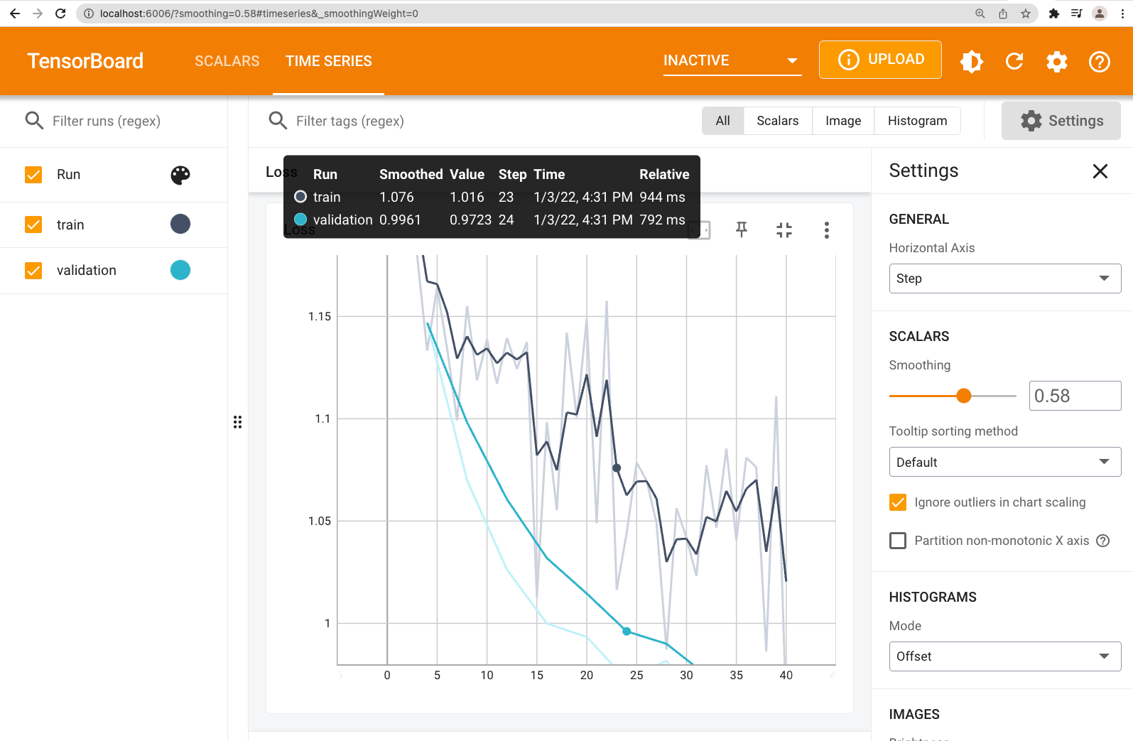
7. Analyze training logs with TensorBoard
After the training finishes, TensorBoard logs will be availabile
$ tree logdir/
logdir/
└── iris-example
    ├── train
    │   └── bigdl.tfevents.1641256264.dzlab-2.local
    └── validation
        └── bigdl.tfevents.1641256270.dzlab-2.local

3 directories, 2 files
Make sure TensorBoard is available in your system or install it with
$ conda install -c conda-forge tensorboard
Now we can visualize the training logs
$ tensorboard --logdir=logdir/iris-example/
TensorFlow installation not found - running with reduced feature set.

NOTE: Using experimental fast data loading logic. To disable, pass
    "--load_fast=false" and report issues on GitHub. More details:
    https://github.com/tensorflow/tensorboard/issues/4784

Serving TensorBoard on localhost; to expose to the network, use a proxy or pass --bind_all
TensorBoard 2.7.0 at http://localhost:6006/ (Press CTRL+C to quit)
Then, visit TensorBoard UI at http://localhost:6006/
8. Evaluate the model against a hold up dataset
val evalResult = model.evaluate(evalRDD, 8)
val evalMetrics = evalResult.map{case (result: ValidationResult, method: ValidationMethod[Float]) =>
    (method.toString(), result.result()._1.toDouble)
}.toMap
Printing the evaluation metrics with println(evalMetrics) will return something like Map(Loss -> 1.0945806503295898).
9. Save to disk
We can save the model and its parameters in a binary format locally, on HDFS or on S3 simply
model.saveModule("/path/to/model", overWrite = true)
10. Load the model from disk
A saved model can be loaded again and used to run predictions
val model2 = Module.loadModule[Float]("/path/to/model")
val predictions = model2.predict(evalData, 4)