
Build and Train a MiniGPT with JAX
20 Aug 2026 by dzlabIn this article, we will build a workflow for training a language-model using JAX ecosystem. Specifically, we will build a compact GPT-style language model with JAX and Flax NNX, train it on a small text dataset called TinyStories, use Orbax for checkpointing, and run text generation from the restored model.
flowchart LR
    A[TinyStories text] --> B[GPT-2 tokenizer]
    B --> C[Fixed-length token batches]
    C --> D[MiniGPT decoder]
    D --> E[Optax loss and optimizer]
    E --> F[NNX JIT training step]
    F --> G[Orbax checkpoint]
    G --> H[Text generation]

    classDef data fill:#e8f4ff,stroke:#1677b9,color:#0b2d42;
    classDef preprocess fill:#fff4cc,stroke:#b58100,color:#3d2b00;
    classDef model fill:#efe8ff,stroke:#6a45b8,color:#241340;
    classDef train fill:#ffe8ec,stroke:#c43e5c,color:#4b1420;
    classDef artifact fill:#e8f8ef,stroke:#23834d,color:#0e3d24;
    classDef inference fill:#fdeee2,stroke:#bf5b17,color:#4a2105;
    class A data;
    class B,C preprocess;
    class D model;
    class E,F train;
    class G artifact;
    class H inference;
Although the model is small, we still can cover the core pieces of a language model: the decoder architecture, tokenized data pipeline, differentiable training step, checkpoint handling, and an inference loop that turns token logits back into text.
The complete source material is available in Build and Train an LLM with JAX.
Setup
First, install the following Python dependencies:
jax==0.6.2
flax==0.10.7
grain==0.2.13
tiktoken==0.4.0
ipywidgets==8.1.8
typing-extensions==4.15.0
jupyter==1.1.1
matplotlib==3.10.8
Note: If Orbax was not pulled in by the Flax/JAX stack, it can be install by adding explicitly these dependencies
optaxandorbax-checkpoint.
Then, imports the libraries and set global constants:
import jax
import jax.numpy as jnp
import flax.nnx as nnx
import grain.python as grain
import optax
import tiktoken
from pathlib import Path

tokenizer = tiktoken.get_encoding("gpt2")

vocab_size = tokenizer.n_vocab
maxlen = 128
embed_dim = 192
num_heads = 6
num_transformer_blocks = 6
feed_forward_dim = 512
batch_size = 32
num_epochs = 3
We will use these libraries to implement various stages of the training workflow:
| Stage | Library | Role |
|---|---|---|
| Model definition | Flax NNX | Defines stateful modules for embeddings, attention blocks, and the output projection. |
| Array computation | JAX | Handles array operations, automatic differentiation, vectorization, and JIT compilation. |
| Data loading | Grain | Samples stories and batches fixed-shape token arrays. |
| Optimization | Optax | Provides cross-entropy, AdamW, and a warmup cosine learning-rate schedule. |
| Checkpointing | Orbax | Saves and restores model state as a PyTree. |
Model Architecture
The model we will be building is small in size, a 20.2M parameter decoder with the GPT-2 tokenizer vocabulary, a context length of 128 tokens, and six causal attention blocks. The different model parameters are as follows:
| Setting | Value |
|---|---|
| Vocabulary size | 50,257 |
| Context length | 128 tokens |
| Embedding dimension | 192 |
| Attention heads | 6 |
| Transformer blocks | 6 |
| Feed-forward dimension setting | 512 |
| Parameters | 20,212,608 |
The first block of the model is the embedding layer that combines token identity with position. The token embedding maps GPT-2 token IDs into dense vectors, while the positional embedding gives the model an order signal. It is defined as:
class TokenAndPositionEmbedding(nnx.Module):
    def __init__(self, maxlen, vocab_size, embed_dim, *, rngs):
        self.token_emb = nnx.Embed(vocab_size, embed_dim, rngs=rngs)
        self.pos_emb = nnx.Embed(maxlen, embed_dim, rngs=rngs)

    def __call__(self, x):
        seq_len = x.shape[1]
        positions = jnp.arange(seq_len)[None, :]
        return self.token_emb(x) + self.pos_emb(positions)
The attention block uses Flax NNX’s MultiHeadAttention. A causal mask prevents each token from attending to future tokens, which is the core rule that makes next-token prediction work. It is defined as:
class TransformerBlock(nnx.Module):
    def __init__(self, embed_dim, num_heads, ff_dim, *, rngs):
        self.attention = nnx.MultiHeadAttention(
            num_heads=num_heads,
            in_features=embed_dim,
            qkv_features=embed_dim,
            out_features=embed_dim,
            decode=False,
            rngs=rngs,
        )

    def __call__(self, x, mask=None):
        attn_out = self.attention(x, mask=mask)
        x = x + attn_out
        return x
The full MiniGPT model wires together embeddings, repeated attention blocks, and a final vocabulary projection. It returns one logit vector per position in the input sequence. It is defined as:
class MiniGPT(nnx.Module):
    def __init__(self, maxlen, vocab_size, embed_dim, num_heads,
                 feed_forward_dim, num_transformer_blocks, *, rngs):
        self.maxlen = maxlen
        self.embedding = TokenAndPositionEmbedding(
            maxlen, vocab_size, embed_dim, rngs=rngs
        )
        self.transformer_blocks = [
            TransformerBlock(embed_dim, num_heads, feed_forward_dim, rngs=rngs)
            for _ in range(num_transformer_blocks)
        ]
        self.output_layer = nnx.Linear(
            embed_dim, vocab_size, use_bias=False, rngs=rngs
        )

    def causal_attention_mask(self, seq_len):
        return jnp.tril(jnp.ones((seq_len, seq_len)))

    def __call__(self, token_ids):
        seq_len = token_ids.shape[1]
        mask = self.causal_attention_mask(seq_len)
        x = self.embedding(token_ids)

        for block in self.transformer_blocks:
            x = block(x, mask=mask)

        return self.output_layer(x)
During training/inference, as depicted by the diagram below, the data will flow through the model in batches of token IDs with shape batch_size x maxlen. The model, first turns those IDs into embeddings, then applies a succession of causal decoder blocks, and finally projects every position back to the GPT-2 vocabulary. During training, the resulting logits are compared with the same batch shifted one token to the left.
flowchart LR
    B["Token batch<br/>batch_size x maxlen"] --> T["Token embedding<br/>batch_size x maxlen x embed_dim"]
    B --> P["Position IDs<br/>1 x maxlen"]
    P --> PE["Position embedding<br/>1 x maxlen x embed_dim"]
    T --> S["Add token + position embeddings"]
    PE --> S
    P --> M["Causal attention mask<br/>maxlen x maxlen"]
    S --> X["Decoder block 1"]
    M --> X
    X --> R["Decoder blocks 2..6"]
    M --> R
    R --> O["Vocabulary projection"]
    O --> L["Logits<br/>batch_size x maxlen x vocab_size"]
    B --> Y["Shifted targets<br/>batch_size x maxlen"]
    L --> C["Cross-entropy loss"]
    Y --> C

    classDef input fill:#e8f4ff,stroke:#1677b9,color:#0b2d42;
    classDef embedding fill:#fff4cc,stroke:#b58100,color:#3d2b00;
    classDef mask fill:#eef2f7,stroke:#64748b,color:#102a43;
    classDef decoder fill:#efe8ff,stroke:#6a45b8,color:#241340;
    classDef output fill:#e8f8ef,stroke:#23834d,color:#0e3d24;
    classDef loss fill:#ffe8ec,stroke:#c43e5c,color:#4b1420;
    class B,P,Y input;
    class T,PE,S embedding;
    class M mask;
    class X,R,O decoder;
    class L output;
    class C loss;
Training Data
The training data used here is a small dataset of short stories where each story ends with <|endoftext|> delimiter. There are 1,000 stories; with the shortest story has 61 whitespace-separated words, the longest has 837, and the average is about 184 words.
First, we need to define a helper function to read stories text file:
def load_stories_from_file(file_path, max_stories=None):
    text = Path(file_path).read_text(encoding="utf-8", errors="replace")
    stories = [
        story.strip() + "<|endoftext|>"
        for story in text.split("<|endoftext|>")
        if story.strip()
    ]

    if max_stories is not None:
        return stories[:max_stories]

    return stories
During transformation, each story becomes a fixed-length token sequence. Longer stories are truncated to the context length, and shorter stories are right-padded with zeros. Right padding matters because the generation function later uses the same alignment when it predicts the next token from a shorter prompt. This is implemented as follows:
class StoryDataset:
    def __init__(self, stories, maxlen, tokenizer):
        self.stories = stories
        self.maxlen = maxlen
        self.tokenizer = tokenizer
        self.end_token = tokenizer.encode(
            "<|endoftext|>",
            allowed_special={"<|endoftext|>"},
        )[0]

    def __len__(self):
        return len(self.stories)

    def __getitem__(self, idx):
        story = self.stories[idx]
        tokens = self.tokenizer.encode(
            story,
            allowed_special={"<|endoftext|>"},
        )

        if len(tokens) > self.maxlen:
            tokens = tokens[:self.maxlen]

        tokens.extend([0] * (self.maxlen - len(tokens)))
        return tokens
Next, we use the Grain library to implement a Data loader that will create batches for training from the raw text.
def create_dataloader(stories, tokenizer, maxlen, batch_size,
                      shuffle=False, num_epochs=1, seed=42,
                      worker_count=0):
    dataset = StoryDataset(stories, maxlen, tokenizer)
    estimated_batches = len(dataset) // batch_size

    sampler = grain.IndexSampler(
        num_records=len(dataset),
        shuffle=shuffle,
        seed=seed,
        shard_options=grain.NoSharding(),
        num_epochs=num_epochs,
    )

    dataloader = grain.DataLoader(
        data_source=dataset,
        sampler=sampler,
        operations=[
            grain.Batch(batch_size=batch_size, drop_remainder=True)
        ],
        worker_count=worker_count,
    )

    return dataloader, estimated_batches
The parameter
drop_remainder=Truehelps keep every batch of the same shape and makes JIT compilation simpler.
The transformation is depicted by the following diagram: load one story, encode it with the GPT-2 tokenizer, normalize it to maxlen, and let Grain stack those rows into a training batch.
flowchart LR
A["Raw story text<br/>One day, a little girl named Lily..."] --> B["Story record<br/>append <|endoftext|>"]
B --> C["GPT-2 tokenizer<br/>tokenizer.encode(..., allowed_special=...)"]
C --> D["Token IDs<br/>[3198, 1110, 11, 257, 1310, 2576, ...]"]
D --> E{"More than maxlen tokens?"}
E -- yes --> F["Truncate<br/>tokens[:128]"]
E -- no --> G["Keep encoded story"]
F --> H["Right pad with 0<br/>until length = 128"]
G --> H
H --> I["StoryDataset row<br/>[token_0, ..., token_127]"]
I --> J["Grain batch<br/>batch_size x maxlen"]
classDef text fill:#e8f4ff,stroke:#1677b9,color:#0b2d42;
classDef tokenize fill:#fff4cc,stroke:#b58100,color:#3d2b00;
classDef branch fill:#fdeee2,stroke:#bf5b17,color:#4a2105;
classDef shape fill:#e8f8ef,stroke:#23834d,color:#0e3d24;
classDef batch fill:#efe8ff,stroke:#6a45b8,color:#241340;
class A,B text;
class C,D tokenize;
class E,F,G branch;
class H,I shape;
class J batch;
Training Loop
For training the model we need first to define the training objective which is next-token prediction. Our model receives an input sequence and learns to predict the target sequence. The target is the same token sequence shifted left by one position which can be implemented in JAX as:
prep_target_batch = jax.vmap(
    lambda tokens: jnp.concatenate((tokens[1:], jnp.array([0])))
)
Next we define the loss function for the training. Using Optax we compute token-level softmax cross-entropy and averages it across the batch.
def loss_fn(model, batch):
    inputs, targets = batch
    logits = model(inputs)
    loss = optax.softmax_cross_entropy_with_integer_labels(
        logits, targets
    ).mean()
    return loss, logits
Next we step the Learning Rate schedule (a warmup cosine schedule) and the optimizer (AdamW):
total_steps = batches_per_epoch * num_epochs
warmup_steps = max(1, total_steps // 10)

lr_schedule = optax.warmup_cosine_decay_schedule(
    init_value=0.0,
    peak_value=3e-4,
    warmup_steps=warmup_steps,
    decay_steps=total_steps,
    end_value=1e-5,
)

optimizer = nnx.Optimizer(
    model,
    optax.adamw(learning_rate=lr_schedule, weight_decay=0.01),
)
Next we define the training step with @nnx.jit to compile it. We perform a forward pass, use nnx.value_and_grad to compute the loss and gradients, the use metrics.update to record training metrics, and finally optimizer.update to mutate the model parameters through the NNX optimizer wrapper.
@nnx.jit
def train_step(model, optimizer, metrics, batch):
    grad_fn = nnx.value_and_grad(loss_fn, has_aux=True)
    (loss, logits), grads = grad_fn(model, batch)

    metrics.update(loss=loss, logits=logits, labels=batch[1])
    optimizer.update(grads)
Finally, we defind the training loop: convert each Grain batch into JAX integer arrays, builds the shifted targets, calls the JIT-compiled training step, and record the metrics:
metrics_history = {"train_loss": []}

for epoch in range(num_epochs):
    step = 0
    for batch in text_dl:
        input_batch = jnp.array(jnp.array(batch).T).astype(jnp.int32)
        target_batch = prep_target_batch(input_batch).astype(jnp.int32)

        train_step(model, optimizer, metrics, (input_batch, target_batch))

        if (step + 1) % 2 == 0:
            for metric, value in metrics.compute().items():
                metrics_history[f"train_{metric}"].append(value)
            metrics.reset()

        step += 1
The following diagram puts together the different parts of the training loop:
flowchart LR
    A["Grain DataLoader<br/>fixed-size token batches"] --> B["Epoch loop"]
    B --> C["Fetch next batch"]
    C --> D["Convert to JAX int32<br/>input_batch"]
    D --> E["Shift tokens left<br/>target_batch"]
    E --> F["JIT train_step"]
    F --> G["MiniGPT forward pass<br/>logits"]
    G --> H["Cross-entropy<br/>logits vs targets"]
    H --> I["value_and_grad<br/>loss + gradients"]
    I --> J["AdamW update<br/>model parameters"]
    I --> K["metrics.update<br/>loss history"]
    J --> L{"More batches?"}
    K --> L
    L -- yes --> C
    L -- no --> M{"More epochs?"}
    M -- yes --> B
    M -- no --> N["Trained model<br/>checkpoint-ready"]

    classDef data fill:#e8f4ff,stroke:#1677b9,color:#0b2d42;
    classDef loop fill:#fdeee2,stroke:#bf5b17,color:#4a2105;
    classDef tensor fill:#fff4cc,stroke:#b58100,color:#3d2b00;
    classDef compute fill:#efe8ff,stroke:#6a45b8,color:#241340;
    classDef update fill:#ffe8ec,stroke:#c43e5c,color:#4b1420;
    classDef output fill:#e8f8ef,stroke:#23834d,color:#0e3d24;
    class A,C data;
    class B,L,M loop;
    class D,E tensor;
    class F,G,H,I compute;
    class J,K update;
    class N output;
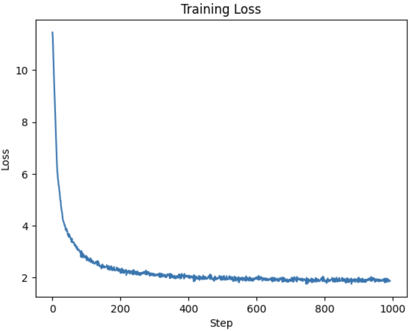
When running this loop over 2,000,000 stories for 3 epochs, the loss drops quickly in the early steps and then flattens near 2.
Checkpointing
Once the model has trained, we can use Orbax to save the NNX model state:
from pathlib import Path
import orbax

checkpoint_path = Path.cwd() / "small_checkpoint.orbax"
checkpointer = orbax.checkpoint.PyTreeCheckpointer()
checkpointer.save(checkpoint_path, nnx.state(model), force=True)
Then during inference we can restore the checkpoint onto a CPU device:
from orbax import checkpoint
from jax.sharding import SingleDeviceSharding

cpu_device = jax.devices("cpu")[0]
cpu_sharding = SingleDeviceSharding(cpu_device)

restore_args = jax.tree_util.tree_map(
    lambda _: checkpoint.ArrayRestoreArgs(sharding=cpu_sharding),
    nnx.state(model),
)
Note: A checkpoint is not just a flat file, it is structured model state, and each array needs sharding information when it is loaded.
Inference
During inference, we simply loop around next-token prediction: keep track of the growing token list, slices the latest model context, right-pads if the prompt is shorter than maxlen, runs the model, and selects the next token.
def generate_text(model, start_tokens, max_new_tokens=50, temperature=1.0):
    tokens = list(start_tokens)

    for _ in range(max_new_tokens):
        context = tokens[-model.maxlen:]
        actual_len = len(context)

        if actual_len < model.maxlen:
            context = context + [0] * (model.maxlen - actual_len)

        context_array = jnp.array(context)[None, :]
        logits = model(context_array)
        next_token_logits = logits[0, actual_len - 1, :] / temperature
        next_token = int(jnp.argmax(next_token_logits))

        if next_token == tokenizer.encode(
            "<|endoftext|>",
            allowed_special={"<|endoftext|>"},
        )[0]:
            break

        tokens.append(next_token)

    return tokenizer.decode(tokens)
Wrap the tokenizer and generator in a small convenience function:
def generate_story(model, story_prompt, temperature=1.0, max_new_tokens=50):
    start_tokens = tokenizer.encode(story_prompt)[:maxlen]
    return generate_text(
        model,
        start_tokens,
        max_new_tokens=max_new_tokens,
        temperature=temperature,
    )
The restored model generates a short TinyStories-like continuation:
Once upon a time a big bear ops were in the forest. He was very happy and he was always looking for something to do. One day, he saw a big, shiny rock
Depending on the input prompt, the model may generate garbage or an imperfect text that look like a story, but this is expected considering how small the model is as well as the training.
I hope you enjoyed this article. Feel free to leave a comment or reach out on twitter @bachiirc.