
Audio Classification using DeepLearning for Image Classification
13 Nov 2018 by dzlabAudio Classification using Image Classification
The following tutorial walk you through how to create a classfier for audio files that uses Transfer Learning technique form a DeepLearning network that was training on ImageNet.
YES we will use image classification to classify audios, deal with it.
Data
Audio Dataset
We will be using Freesound General-Purpose Audio Tagging dataset which can be grapped from Kaggle - link.
In this dataset, there is a set of 9473 wav files for training in the audio_train folder and a set of 9400 wav files that constitues the test set.
Sounds in this dataset are unequally distributed in the following 41 categories of the Google’s AudioSet Ontology:
"Acoustic_guitar", "Applause", "Bark", "Bass_drum", "Burping_or_eructation", "Bus", "Cello", "Chime", "Clarinet", "Computer_keyboard", "Cough", "Cowbell", "Double_bass", "Drawer_open_or_close", "Electric_piano", "Fart", "Finger_snapping", "Fireworks", "Flute", "Glockenspiel", "Gong", "Gunshot_or_gunfire", "Harmonica", "Hi-hat", "Keys_jangling", "Knock", "Laughter", "Meow", "Microwave_oven", "Oboe", "Saxophone", "Scissors", "Shatter", "Snare_drum", "Squeak", "Tambourine", "Tearing", "Telephone", "Trumpet", "Violin_or_fiddle", "Writing"
Once you downloaded this audio dataset, we can then start playing with
Data PreProcessing
These audio files are uncompressed PCM 16 bit, 44.1 kHz, mono audio files which make just perfect for a classification based on spectrogram. We will be using the very handy python library librosa to generate the spectrogram images from these audio files. Another option will be to use matplotlib specgram().
The following snippet converts an audio into a spectrogram image:
def plot_spectrogram(audio_path):
y, sr = librosa.load(audio_path, sr=None)
# Let's make and display a mel-scaled power (energy-squared) spectrogram
S = librosa.feature.melspectrogram(y, sr=sr, n_mels=128)
# Convert to log scale (dB). We'll use the peak power (max) as reference.
log_S = librosa.power_to_db(S, ref=np.max)
# Make a new figure
plt.figure(figsize=(12,4))
# Display the spectrogram on a mel scale
# sample rate and hop length parameters are used to render the time axis
librosa.display.specshow(log_S, sr=sr, x_axis='time', y_axis='mel')
# Put a descriptive title on the plot
plt.title('mel power spectrogram')
# draw a color bar
plt.colorbar(format='%+02.0f dB')
# Make the figure layout compact
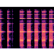
plt.tight_layout()For instance, the sounds of a Drawer that opens or closes looks like:
In our case, we need to store those images, unfortunate we have to plot them then store the plot. This is going to be very slow considering that we few thousands images. Following is the snippet for storing the images:
def save_spectrogram(audio_fname, image_fname):
    y, sr = librosa.load(audio_fname, sr=None)
    S = librosa.feature.melspectrogram(y, sr=sr, n_mels=128)
    log_S = librosa.power_to_db(S, ref=np.max)
    librosa.display.specshow(log_S, sr=sr, x_axis='time', y_axis='mel')
    fig1 = plt.gcf()
    plt.axis('off')
    plt.show()
    plt.draw()
    fig1.savefig(image_fname, dpi=100)

def audio_to_spectrogram(audio_dir_path, image_dir_path=None):
    for paths in batch(audio_dir_path.ls(), 100):
        for audio_path in paths:
            audio_filename = get_filename(audio_path)
            image_fname = audio_filename.split('.')[0] + '.png'
            if image_dir_path:
                image_fname = image_dir_path.as_posix() + '/' + image_fname
            if Path(image_fname).exists(): continue
            print(image_fname)
            #plot_spectrogram(image_fname)
            try:
                save_spectrogram(audio_path.as_posix(), image_fname)
            except ValueError as verr:
                print('Failed to process %s %s' % (image_fname, verr))
        # wait between every batch for xyz seconds
        time.sleep(10)
Once the spectrogram files are generated for both training and test sets, we can have a look at them.
- load the labels from the csv file and have a look to the first 5
View data
# get the labeled data from the `train.csv` file
df_train = pd.read_csv('path/to/freesound/train.csv'); df_train.head()
fname label manually_verified
0 00044347.wav Hi-hat 0
1 001ca53d.wav Saxophone 1
2 002d256b.wav Trumpet 0
3 0033e230.wav Glockenspiel 1
4 00353774.wav Cello 1
# get the labels of the audio dataset
labels = df_train['label']; labels[:5]
0 Hi-hat
1 Saxophone
2 Trumpet
3 Glockenspiel
4 Cello
Name: label, dtype: object
# get the filenames of all spectrogram images
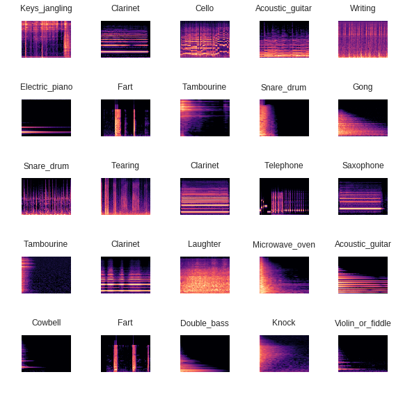
fnames = sorted(image_train_path); fnames[:5]Now we can have a look at the data which will be piped into the DL model Note: there is no need to apply any transformation (cropping, flipping, rotating, light, etc.) to the images we will be classiying. In fact, they are spectrogram and will be always generate same way, unlike the images that someone would take with a camera where the condition can change drastically.
np.random.seed(42)
data = ImageDataBunch.from_lists(path, fnames, labels, ds_tfms=None, size=224, bs=bs)
data.normalize(imagenet_stats)
data.show_batch(rows=5, figsize=(8,8))
Following is an example of spectrograms with their corresponding labels:
DeepLearning
Now the DL part can finally start
Model training
First, create a pre-trained ResNet-34 based model, and look for best learning rate that we will choose later when training the final layers of this network.
learn = create_cnn(data, models.resnet34, metrics=error_rate)
learn.lr_find()
learn.recorder.plot()
Plotting the recorded learning rate will give us somethine like this:
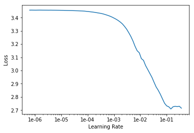
Now we can training the FeedFordward last layers with the learning slice that we choosed wisely from the previous plot. Choose the ones that bounds a steep decreasing plot.
lr=1e-2
learn.fit_one_cycle(5, slice(lr))

Total time: 36:59
epoch  train_loss  valid_loss  error_rate
1      2.573095    1.728513    0.476064    (28:29)
2      1.685420    1.314066    0.367553    (02:10)
3      1.244419    1.147185    0.324468    (02:08)
4      0.924578    1.065614    0.305851    (02:04)
5      0.744983    1.049067    0.295213    (02:06)
We can keep training the entire net after unfreezing for more epochs as follows:
learn.unfreeze()
learn.fit_one_cycle(10, max_lr=slice(1e-5, 1e-4))

Total time: 23:48
epoch  train_loss  valid_loss  error_rate
1      0.692382    1.029194    0.297340    (02:14)
2      0.616119    0.993735    0.280851    (02:09)
3      0.497737    0.958199    0.268617    (02:17)
4      0.342366    0.942322    0.256915    (02:24)
5      0.221545    0.936434    0.261170    (02:26)
6      0.143401    0.885661    0.242553    (02:24)
7      0.091955    0.894207    0.237234    (02:25)
8      0.062393    0.874940    0.231915    (02:26)
9      0.051603    0.870887    0.232979    (02:27)
10     0.046500    0.871038    0.229255    (02:30)
The training technique is based on the one cycle policy, here is the original ResNet paper.
Model Interpretation
interp = ClassificationInterpretation.from_learner(learn)Plot the top losses, i.e. the cases where the model uncorrectly predicted the labels:
interp.plot_top_losses(9, figsize=(15,11))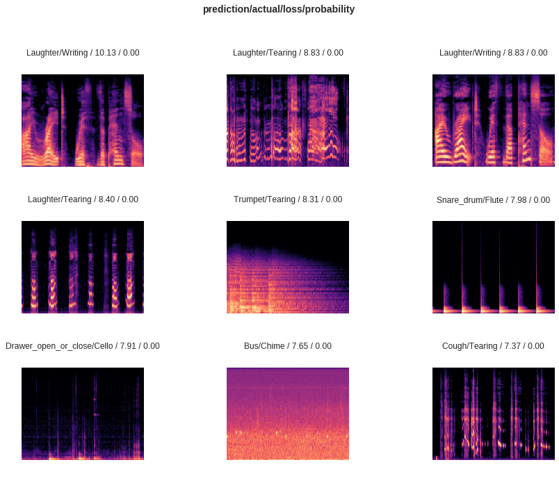
Plot the confusion matrix, i.e. for each orginial label the distribution of number of times the model predicted images from this label to be of one fo the rest classes. The best matrix should have zeros except in the diagonal.
interp.plot_confusion_matrix(figsize=(15,15), dpi=60)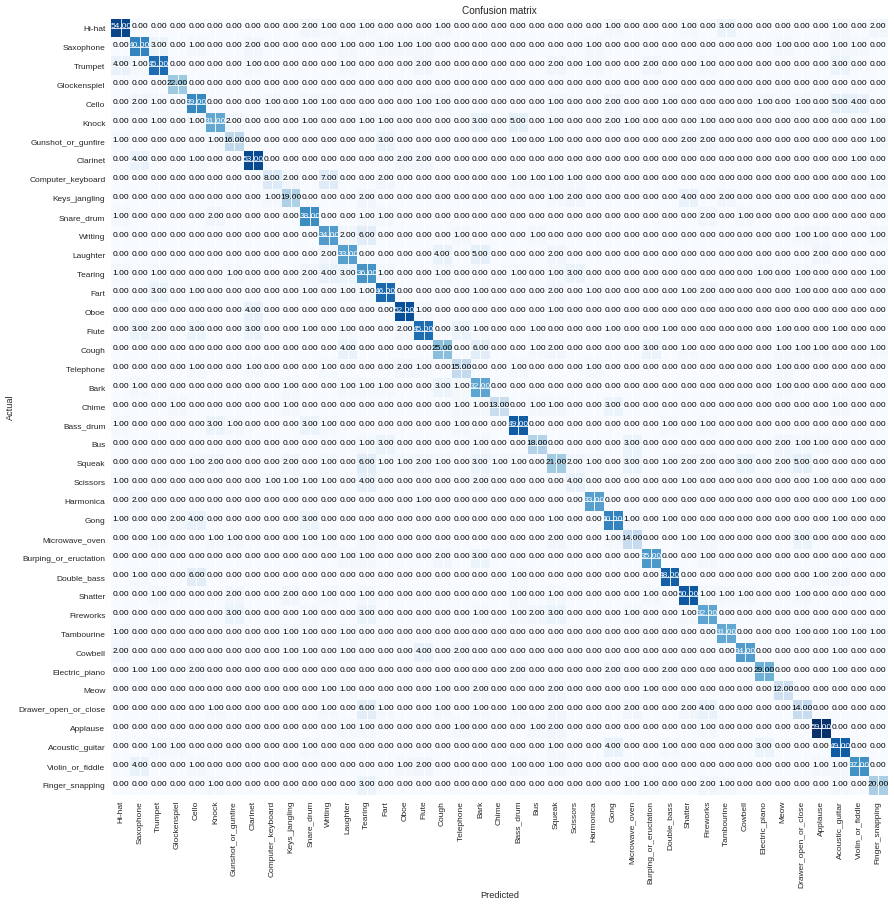
We can perform t-SNE on our model’s output vectors. As these vectors are from the final classification, we would expect them to cluster well.
probs_trans = manifold.TSNE(n_components=2, perplexity=15).fit_transform(preds)
prob_df = pd.DataFrame(np.concatenate((probs_trans, y[:,None]), axis=1), columns=['x','y','labels'])
g = sns.lmplot('x', 'y', data=prob_df, hue='labels', fit_reg=False, legend=False)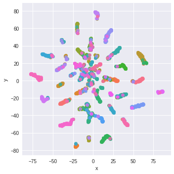
What’s next
An alternative for using spectrogram images is generating Mel-frequency cepstral coefficients (MFCCs). Here is an example of training on MFCC for audio classification - link.
It is also possible to explore other techniques for coding sound, here is nice lecture about this topic - youtube.
Full jupyter notebooks: