Optimizers Visualisation

15 Jun 2019 by dzlab

Vanila Gradient Descent

Gradient descent is by far the most popular class of optmisation algorithms used in Deep Learning. Implemented in all DL libraries as a black box tool for updating neural network weigths.

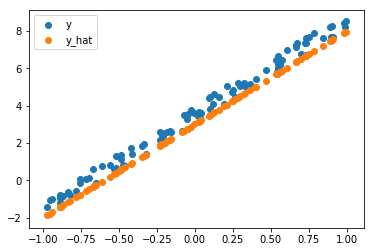
This post explores the different gradient-based optimization algorithms, how they work and look like, their strengths and weaknesses. We will be using a simple regression problem with one variable \(x\) a one target variable \(y\), the dataset that looks like this:

On a high level, Gradient Desent (GD) is an iterative optimization algorithm for an objective function (also called cost function) \(J(\theta)\) parametrized by \(\theta\). Usually, a learning rate is associated with (GD), this hyper parameter is used to control the amount \(\theta\) will be updated with a every step/iteration of the optimization.

In our case, the optimization problem aims to find best values for two parameters \(\theta_0\) and \(\theta_1\) such the predicted \(\hat{y}\) (defiend as \(\hat{y} = \theta_0 + \theta_1 * x\)) is as close as possible to the real values of \(y\). The closiness is measured by the lost function that GD tries to optimise. The most commonly used cost functions are:

Loss function	Equation	Our case
Mean Square Error	\(\frac{1}{n} \sum_{i}^{n} (y_i - \hat{y}_i)^2\)	\(\frac{1}{n} \sum_{i}^{n} (y_i - \theta_0 - \theta_1 * x_i)^2\)
Mean Square Root Error	\(\sqrt{ \frac{1}{n} \sum_{i}^{n} (y_i - \hat{y}_i)^2 }\)	\(\sqrt{ \frac{1}{n} \sum_{i}^{n} (y_i - \theta_0 - \theta_1 * x_i)^2 }\)
Mean Absolute Error	\(\frac{1}{n} \sum_{i}^{n} |y_i - \hat{y}_i|\)	\(\frac{1}{n} \sum_{i}^{n} |y_i - \theta_0 - \theta_1 * x_i|\)

For our problem, the shape of those loss function looks as follows:

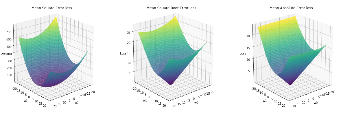
You can notice that Mean Square Error is on a different scale that the other two loss functions, and that the square root in Mean Square Root Error is effectively bringing the loss back to regular scale.

The main equation used by Gradient descent to update the parameter \(\theta\) given a learning rate \(\eta\) and the derivitate of the cost function \(\nabla_{\theta} J(\theta)\) is as follows:

\[\theta = \theta - \eta \nabla_{\theta} J(\theta)\]

The basic version of Gradient descent computes the gradient for the cost function over the entire dataset. The most commonly used variation is Mini-batch gradient descent which uses same equation but calculates the gradients on one batch at a time.

Limitations

This basic form of optimization comes with a lot of flaws

• The convergance of the optimization is very sensible to the learning rate \(\eta\), a small learning rate leads to very slow convergence, a large learning rate leads to a divergence in most cases.
• It uses the same learning rate for all parameters regardless of any specificity (e.g. associated layer number, pre-trained layer or not).
• It is very sensible to local minima, which is very common for cost function of neural networks that tend to be non-convex.
• The use of any learning rate scheduling (i.e. adapting \(\eta\) on pre-defined schedules) is not straightforward, may become ineffective depending on the dataset characteristics.

Optimization tweaks

To overcome those limitations, different tweaks and ideas were introduced to the basic Mini-batch GD.

Weight Decay

A regularization form, unlike the L2 regularization that adds the sum of the squared parameters to the loss function as a way to penalize large params. Weight Decay (WD) adds a proportion of the weights (i.e. \(wd * \theta\)) to the gradient leading to a better numerical unstability as a result of avoiding summing big numbers. The weight update funtion becomes:

\[\theta = \theta - \eta (\nabla_{\theta} J(\theta) + wd * \theta)\]

Momentum

Momentum is a convergence acceleration tweak. It helps GD navigates curves which are steep in one direction and not very on others (i.e. local optimal) where usually GD will oscillated. Technically, Momentum adds to the gradients a fraction \(\beta\) (usually equal to 0.9) of the previous upate applied to the weights. The weight update function becomes:

\[m_{t} = \beta m_{t-1} + \eta \nabla_{\theta} J(\theta)\] \[\theta_{t+1} = \theta_{t} - m_{t}\]

Adam

Adaptive Moment Estimation (Adam) computes adaptive learning rates which are different per parameter. It keep tracks of:

• \(v_{t}\) which is a vector holding the exponential decaying average of previous squared gradients.
• \(m_{t}\) which is a vector holding the exponential decaying average of previous gradients (simialrly to momentum).

Mathematically, both are defined as follows:

\[m_{t} = \beta_1 m_{t-1} + (1 - \beta_1) \nabla_{\theta} J(\theta)\] \[v_{t} = \beta_2 v_{t-1} + (1 - \beta_2) \nabla_{\theta} J(\theta)^2\]

To avoid having \(v_{t}\) and \(m_{t}\) been biased to 0 during their initial steps, the authors of Adam propose:

\[\hat{m_t} = \frac{m_t}{1 - \beta_1}\] \[\hat{v_t} = \frac{v_t}{1 - \beta_2}\]

The final equation for the gradient updates become:

\[\theta_{t+1} = \theta_{t} - \frac{\eta}{\sqrt{\hat{v_t}} + \epsilon} \hat{m_t}\]

Usually, \(\beta_1\) is 0.9, \(\beta_2\) is 0.999, and \(\epsilon\) is a small value \(10^8\).

LAMB

Layer-wise Adaptive Moments optimizer for Batch training (LAMB) (see link) aims to update the weights at layer \(l\) at batch \(t\) as follows:

\(g^{l}_{t} = \nabla_{\theta} J(\theta^{l}_{t-1}, x_{t})\)

\(m^{l}_{t} = \beta_1 m^{l}_{t-1} + (1 - \beta_1) g^{l}_{t}\)

\(v^{l}_{t} = \beta_2 v^{l}_{t-1} + (1 - \beta_2) g^{l}_{t} \odot g^{l}_{t}\)

\(\hat{m}^{l}_{t} = \frac{m^{l}_{t}}{1-\beta_1^t}\)

\(\hat{v}^{l}_{t} = \frac{v^{l}_{t}}{1-\beta_2^t}\)

\(r_1 = || w^{l}_{t-1} ||_2\)

\(r_2 = || \frac{\hat{m}^{l}_{t}}{\sqrt{\hat{v}^{l}_{t}} + \epsilon} + \lambda w^{l}_{t-1} ||_2\)

\(r = \frac{r_1}{r_2}\)

\(\eta^l = r x \eta\)

\(w^{l}_{t} = w^{l}_{t-1} - \eta^{l} (\frac{\hat{m}^{l}_{t}}{\sqrt{\hat{v}^{l}_{t}} + \epsilon} + \lambda w^{l}_{t-1})\)

Visualization

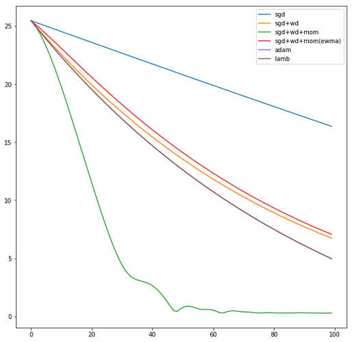
Implementing the different optimization algorithms and applying them to our simple optimization problem using different learning rates \(\eta\).

\(\eta = 0.1\)

Using a learning rate of 0.1 the loss is evaluated at each iteration of the optimization algorithm

Here is an animation showing how the parameters are being updated based on the optmization algorithm

Adam

LAMB

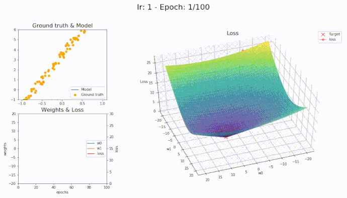
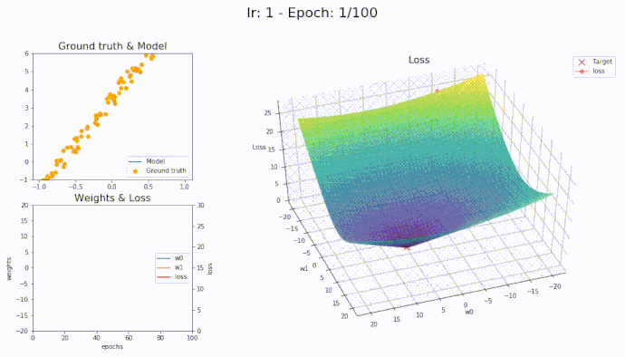
\(\eta = 1\)

Using a learning rate of 1 the loss is evaluated at each iteration of the optimization algorithm

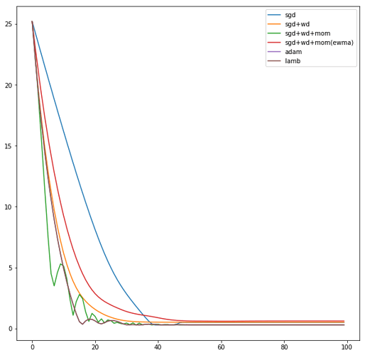
Here is an animation showing how the parameters are being updated based on the optmization algorithm

Adam

LAMB

Conclusion

It seems that with LAMB we can use high learning rate yet the algorithm converge smoothly to the optimal parameters.

The full notebook can be found here.