fastai's Practical Deep Learning For Coders, Part 1

20 Dec 2018 by dzlab

I recently completed Part 1 of Jeremy Howard’s Practical Deep Learning For Coders. The course span over the course of 7 weeks from October to December, one course a week. All what’s needed to join the course is math background of high-school level, a computer, network connectivity and access to a GPU machine, that’s it! The course videos are recorded during the in-person class at the Data Institute at USF, and freely available on youtube.

The following is an attempt to share my takeaways from the lessons.

Note Expect to have to watch the video lessons over and over to fully understand the materials.

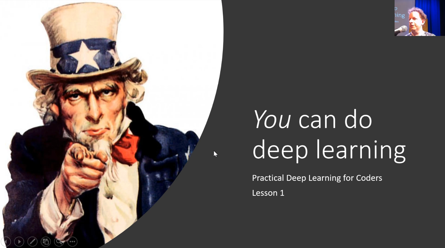
What’s very unique about this course is the focus on the practical side of the learning experince. Right from the very few moments of the course, you will see Deep Learning code, at first you won’t understand what’s it doing, you will not get it unless you’re a Deep Learning expert. But you will be impressed how insanely is it simple to write Deep Learning code to solve problems seconds before the course you would have no idea how they can be solved. You will learn how to take that same code and re-apply it to solve similar problems or even different with the use of the underlying ideas.

Protip: take as mush notes as you can while watching the video lessons, especially when Jeremy says ‘here is the trick’ or the other activation word ‘homework’.

The other very impressive thing about this course is the discussion forum that gathers all the student in one place. Everyone is engaged, very responsive, you should definitely check it. You will find study groups that you could join in your city, examples of other student works that could inspire you. You will find help to get started with the fastai library, to setup your work environemnt in major Cloud providers or answers to any question you could have.

The Course

This is an overview of the course:

Here is some nicely writing lecture notes, kindly shared by Hiromi Suenaga one of the course students.

Lesson 1

Right from first few seconds of the course Jeremy tries to convince you that you can do Deep Learning. Then jumps on a notebook where he would walk you through the cells, run them and explain what is doing and how you could play with it. By the end of the lesson you will be able to build a Resnet based NN for classifying anything.

The homework for this lesson is to apply the same technique on any image classification problem. I myself applied this same notebook to classify Flowers, Birds and even Sounds.

Lesson 2: Computer Vision - Deeper Applications

In this lesson Jeremy takes us deeper into Computer Vision through a teddy bear classification example, walk us through a detailled explication of the solution. Then explains interactively using a notebook what is the algorith Stochastic gradient descent , and how it’s updates the NN weights and get better and better at classifying images.

The lessong ends with the introduction of some technical vocabulary:

• Learning rate: a critical number used to by gradient to control the amount to update the weights.
• Epoch: the number of iterations in the trainning phases. In every run, the trainng goes over all the data points (i.e. every image in the dataset). The number of epochs should not be too high, otherwise the training will see the same images many times and may overfitt and not generalize well.
• Mini-batch: A random set of data points that the training algorithm uses to update weights.
• SGD: Gradient descent using mini-batches.
• Model / Architecture: like ResNet34, generally speaking it can be seen as the mathematical function \(\vec{y} = X\vec{a}\) we are trying to find the parameters to solve.
• Parameters / Coefficients / Weights: Numbers updating after every mini-batch.
• Loss function: a function used to assess how well the predictions \(\hat{y}\) are compared to the real \(y\). In classification problems, we usually uses cross entropy loss, also known as negative log likelihood loss. This penalizes incorrect confident predictions, and correct unconfident predictions.
• Underfitting and Overfitting: underfitting is when the model fails miseralby to predict the outputs in the training set (i.e. was not able to learn well from the data). On the other hand, the model is overfitting when it learns very well to predict the outputs on the training set but fails to generalize on unseen data points (i.e. the loss is very low on training set, but very hign on test dataset).
• Regularization: Regularization techniques help us make sure when we train our model that it’s going to work not only well on the data it’s seen but on the data it hasn’t seen yet.
• Validation Set: at the end of a mini-batch SGD training loop, data from the validation set (i.e. samples not seen during training) are used in the calculation of the loss function and the accuracy to see how good the model is able to generalize.

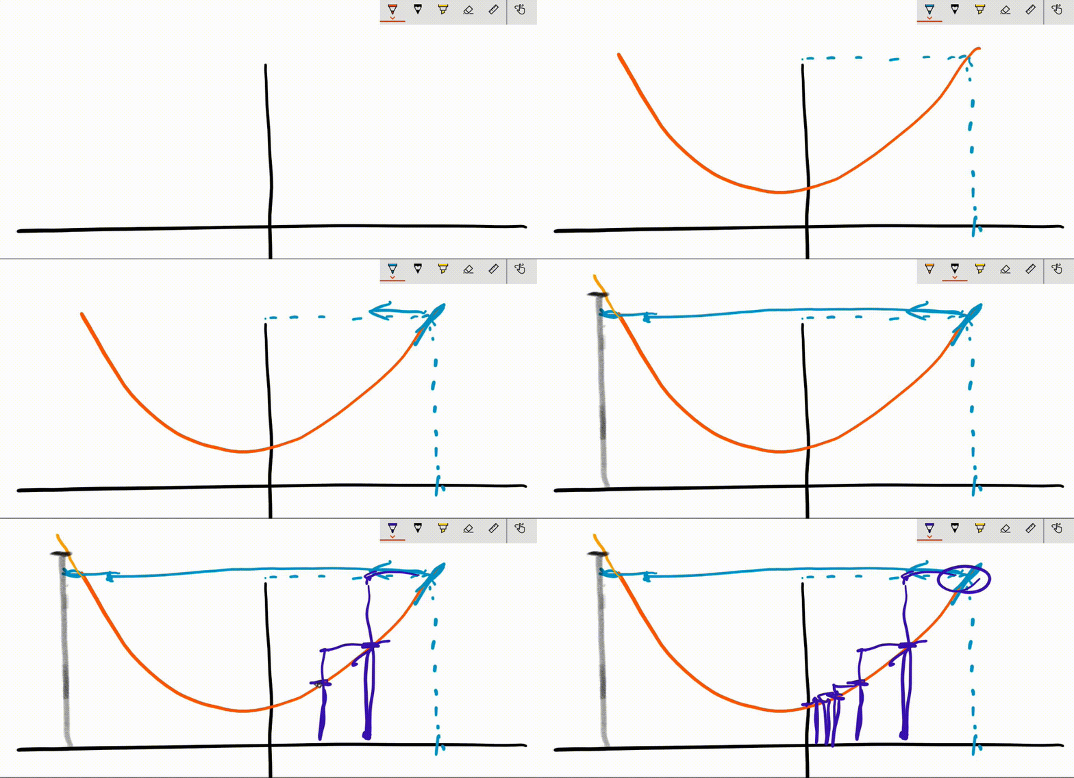
The homework for this lesson is to build an image classification model and deploy it on a web app.

Lesson 3: Multi-label, Segmentation, Image Regression, and More…

The lesson takes time explaining the fancy learning rate plot and how you can interpret it. It also presents a couple of jupyter notebooks for a variety of Deep Learning problems along with the trick that can be used to get good results:

• Multilabel dataset (each image has multiple labels).
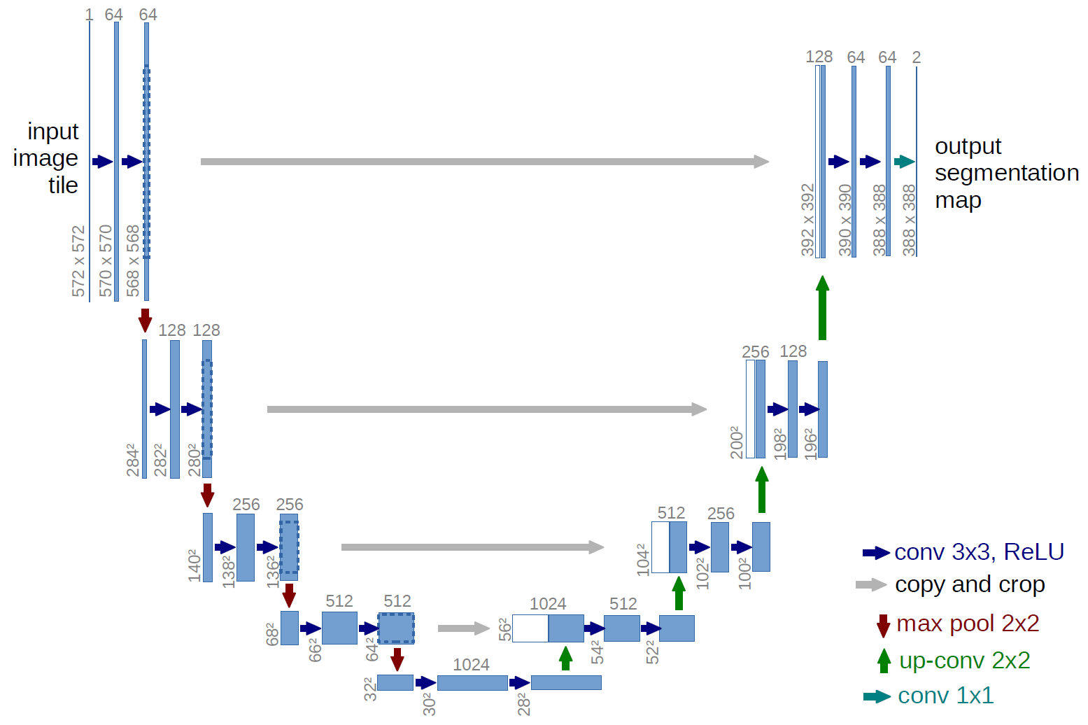
• CamVid dataset (segmentation): the difference is in the use of U-Net with ResNet architecture.
• BIWI dataset (regression, i.e. predict a contiguous number): the difference is in the loss function, in classifiation we tend to use cross entropy, for regression use mean square error.
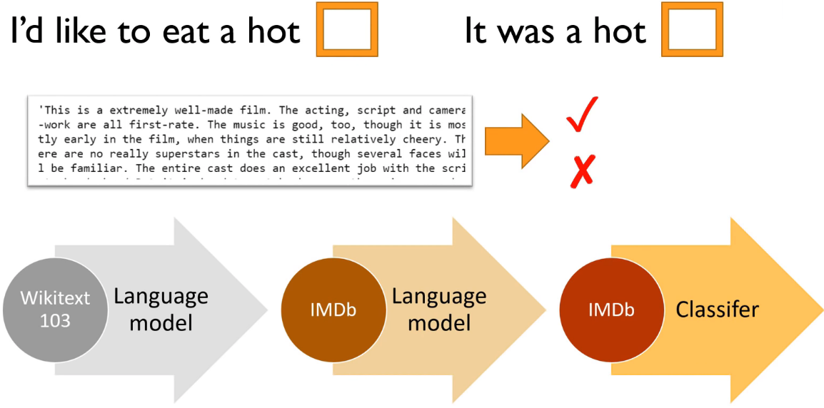
• IMDB dataset: sentiment classification

The homework for this lesson is to reuse those notebooks and build something for segmentation or multi-label classification, etc.

Lesson 4: NLP, Tabular, and Collaborative Filtering

This lesson focuses on Natural Language Processing (NLP) and how to use the idea of transfer learning instead of starting from random weigths to get better results in text related tasks.

Then a use case of using DL to solve tabular data using a simplified version of Adult salary dataset. Finally, an introduction to DL for Collaborative Filtering and prediction of movie rating using the Movielens dataset.

The homework for this lesson is to build an text classification model or collaborative filtering.

Lesson 5: Foundation of Neural Networks

This lesson focus on the describing the main components of deep NN and how to fine tuning a model with descrimitive learning, freezing/unfreezing and transfer learning. It also gives some advices like:

• Do not run for too many epochs, you will overfit for sure.
• Use L2 regularization (also called weight decay when in the gradient form).
• Gradient descent too slow, adam is the combination of momentum plus props.
• For categorical data, use ‘cross entropy’, and make sure your inputs to this loss function are probabilities by using ‘softmax’ function.

Then the course continues on Collaborative Filtering, but this time using a set of Excel spreadsheet to implement it (who on earth would use Excel for DeepLearning, only Jeremy does). The takeaway here is that embedding is an array lookup which is mathimaticay identical to a matrix multiplied by one hot encoded matrix. the underlying features (e.g. movie feautre; movie has John, user feature: user likes john) are called latent features.

Lesson 6: Regularization and CNNs

The lesson covers the tabular data and how to use deep learning for “structured data” such as database tables and spreadsheets, or timeseries. Then the course go to CNNs with an in-depth explication addressing Convolution and Pooling layers, then describes Batch Normalization as a regularisation technique and how to implement such layer from scratch. An interesting regularisation technique that was described is Data Augmentation. The lesson walks through the different transformations available in fastai library to augment image dataset. After that an in-depth walk through Grad-CAM to visualize gradient and how to implement this technique using pytorch hooks with a result similiar to the following picture.

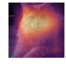
The last part of the lesson is focused on ethical questions related to the use AI to solve day to day problems. Also some concrete examples from Facebook/Meetup of cases where AI algorithm gone wrong.

Lesson 7: RESNETs, UNETs, GANs and RNNs

This is a very very busy lesson. Back to computer vision, Jeremy explains how to implement the ResNet architecture and apply it the MNIST digit classification problem. For once Jeremy didn’t use transfer learning but still get pretty good accuracy with a model trained from scratch. Then back to U-Net which were used for segmentation in lesson 7 but this time to go deeper in the architecture. The interesting part is the use of U-Net for image reconstruction which later is transformed in an implementation of a GAN model with a Generator reposible of retoring an image to its original quality and a Discriminator that tries to recognize original images from restored ones. Also a quick implementation of WGAN is introduced with a use case of generating images of bedrooms starting from noise.

In the last part of the lesson, Jeremy talks introduces recurrent neural network and illustrate how simple it’s to implement them from scratch. Then, he applies it on simple language modeling task on a dataset of numbers in letters. To included RNNs, the lesson talks about GRU and LSTM cells.

The takewawys

By the end of the course, you will understand the fundamental ideas Jeremy cares a lot about, like:

• Transfert learning, the reuse of pre-trained neural networks.
• ResNet are awesome (According to DAWNBench they give the best results), take any architecture and through a ResNet you will get better results.
• Speeding up NN learning with One fit cycle, Cyclical Learning Rate, Descrimitive Learning, Momentum, RMSProp.
• Fine tunning a NN by deleting Layer (usually head) and replace it with ones useful for your problem.
• Random initialization of weights
• Gradullay Freezing & unfreezing layers of the architecture.
• To not be afraid of using big NN and addressing over-fitting with regularization techniques such Weight Decay, Dropout, Batch Normalization.

This course is simply full of practical learning opportunities.