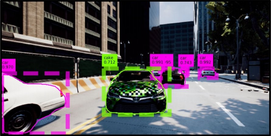
Deep Learning have achieved remarquable results in many areas especially vision where today complex models trained on very large datasets are able to overperform domain experts. Yet those same models can be very vulnerable to attacks that slightly change the input data to fool the model. Those attacks are know as Adversial Attacks and can be performed in a variety of ways (see link1, link2).
Those attacks can be serious with devastating results (e.g. fooling a self-driving), so known how to check that your model is robust against them is crutial before rolling the model to production.

In this article, we will see how to implement one simple and effective Adversial Attack called Fast Gradient Signed Method (FGSM).
FGSM is implemented by performing the following steps:
- Pass an legitimage image over a model and capture the gradients
- Determining the direction (sign) of the gradient at each pixel of the original image
- Using that information create an adversarial pattern in a way to aximize the loss at each pixel
- Multiply this pattern by a small scaling value and apply it (i.e. add or substruct) to the original image
- The result is an Adversial image that looks to the human eye very similar to the original image
Although this attack performs small imperceptible perturbations into an image, we will see in action how this technique can easily fool a pre-trained model.
Before starting, make sure to have OpenCV installed as it will be used for performing the perturbations
#collapse
!pip install opencv-contrib-python
Import the dependencies
#collapse
import cv2
import matplotlib.pyplot as plt
import tensorflow as tf
from tensorflow.keras.applications.nasnet import *
from tensorflow.keras.losses import CategoricalCrossentropy
Load the pre-trained model (in this case NASNetMobile) and freeze its weights so they are not updated after a forward pass.
pretrained_model = NASNetMobile(include_top=True, weights='imagenet')
pretrained_model.trainable = False
We need to define a function to preprocess an image with same preprocessing steps performed on the images used to train the target model (e.g. resizing)
def preprocess(image, target_shape):
    image = tf.cast(image, tf.float32)
    image = tf.image.resize(image, target_shape)
    image = preprocess_input(image)
    image = image[None, :, :, :]
    return image
We also need to define a function that turns the model output probabilities into actual labels
def get_imagenet_label(probabilities):
    return decode_predictions(probabilities, top=1)[0][0]
Define a function to create the adversarial pattern that will be used later to generate the adversial image
def generate_adv_pattern(model, input_image, input_label, loss_function):
    with tf.GradientTape() as tape:
        tape.watch(input_image)
        prediction = model(input_image)
        loss = loss_function(input_label, prediction)

    gradient = tape.gradient(loss, input_image)
    signed_gradient = tf.sign(gradient)
    return signed_gradient
The pattern is nothing but a tensor with the sign of the gradient in each element. i.e., signed_gradient is:
- -1 for negative gradients (i.e. value below 0)
- 1 for positive gradients (i.e. value above 0)
- 0 if the gradient is 0.
We need a legitimate image so we can apply perturbations on it, you can download a test image on your own or use this Pug image
!curl https://image.freepik.com/free-vector/angry-dog-pug-prisoner-graphic-illustration_41984-29.jpg -o dog.jpg
Pass the image through the pretrained model to get output probabilities
image = tf.io.read_file('dog.jpg')
image = tf.image.decode_jpeg(image)
image = preprocess(image, pretrained_model.input.shape[1:-1])
image_probs = pretrained_model.predict(image)
We need to One-hot encode the ground truth label of the original image, then use it to generate an adversarial pattern
cce_loss = CategoricalCrossentropy()
pug_index = 254
label = tf.one_hot(pug_index, image_probs.shape[-1])
label = tf.reshape(label, (1, image_probs.shape[-1]))
disturbances = generate_adv_pattern(pretrained_model, image, label, cce_loss)
pug then look up the corresponding class index in this imagenet class indices - link
Next, we define a utility function to generate an adversial version of an image based on a disturbance/noise and a scalar
def generate_adv_image(image, epsilon, disturbances):
    corrupted_image = image + epsilon * disturbances
    return tf.clip_by_value(corrupted_image, -1, 1)
We also, need another utility function to ensure before plotting that the input tensor in the [0, 255] range, as well as in BGR space, which is the one used by OpenCV
def postprocess_adv_image(adv_image):
    adv_image = adv_image.numpy()[0] * 0.5 + 0.5
    adv_image = (adv_image * 255).astype('uint8')
    return cv2.cvtColor(adv_image, cv2.COLOR_RGB2BGR)
We can use the previous utility function to show what the noise looks like before applying it to the original image
disturbed_image = postprocess_adv_image(disturbances)
plt.imshow(disturbed_image)
plt.axis('off')
plt.title("noise");
Finally, we can put all the previous steps together to perform a series of adversarial attacks different values of epsilon (which is used as noise multiplier).
After that we disply the corresponding adversial example as well the predicted label and confidence provided by the victim model
figure, axis = plt.subplots(2, 3, figsize=(15, 8))
for index, epsilon in enumerate([0, 0.005, 0.01, 0.1, 0.15, 0.2]):
    adv_image = generate_adv_image(image, epsilon, disturbances)
    prediction = pretrained_model.predict(adv_image)
    _, label, confidence = get_imagenet_label(prediction)
    adv_image = postprocess_adv_image(adv_image)
    confidencePct = confidence * 100
    title = f'Epsilon = {epsilon:.3f}, {label} ({confidencePct:.2f}%)'
    row, col = int(index / 3), index % 3
    axis[row, col].imshow(adv_image)
    axis[row, col].set_title(title)
    axis[row, col].axis('off')
As you can be see from the output images and the resulting classification, an imperceptible variation in the pixel values produced a drastically different response from the network.
- For epsilon = 0 (no attack), the label is Pug with a 60.18% confidence
- When epsilon = 0.005 (a very small perturbation), the label changes to Muzzle, with a 98.46% confidence!
- The situation gets worse as we increase the magnitude of epsilon.